Spatio-temporal analysis with GRASS GIS

IHE Delft Institute for Water Education

The Netherlands

Outline

Exercise 1 - Seasonal aggregation and statistical analysis

Objectives

Aim:

The main objective of this exercise is to explore monthly Actual EvapoTranspiration (AETI) and Precipitation (PCP) data from FAO WaPOR over Urmia lake basin, and extract Land cover based statistics for the crop year 2018/2019.

Data provided:

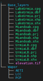
All data provided cover the entire Urmia Lake Basin

Monthly AETI (October 2017 to September 2020) at 250 m resolution
Monthly PCP (October 2017 to September 2020) at 2500 m resolution
Annual Land cover map (2018,2019,2020) at 250 m resolution
SRTM elevation - resampled to 250 m
Base layers - Boundaries of Urmia lake, Urmia lake basin, Miandoab irrigation scheme

For this exercise, we will use some GeoTIFF files obtained from FAO WaPOR and the shape files

Download the data here

Data provided

Step 1: Import data

For this exercise we will use the location/mapset created in previous section: utm38n/ulb_wapor


## Open the Grass GIS in 'utm38n/ulb_wapor' location/mapset
grass78 /mnt/d/grassdata/utm38n/ulb_wapor
## Set the region to ULB
g.region vect=ulb res=250 -a
## remove any Mask
r.mask -r
## We have imported all the vector files (Base_layers) in the previous section.
## Now let us import all the WaPOR data into the grass gis mapset.
## Navigate (cd) to the '' folder provided to you
cd /path/to/Data_ULB/Wapor # change the path to actual path in your computer
## Let us import all the AETI maps first
cd AETI
## List all the maps in the folder
ls
## let us use a 'for' loop to import all the maps in to GRASS GIS mapset in one go.
for i in `ls *.tif`; do
    out=`echo ${i}|cut -d. -f1`
    r.import in=${i} out=${out} extent=region resolution=region
done
## press enter
## Now Let us import all the precipitation maps
cd /path/to/Data_ULB/Wapor/PCP
## let us use a 'for' loop to import all the maps in to GRASS GIS mapset in one go.
for i in `ls *.tif`; do
    out=`echo ${i}|cut -d. -f1`
    r.import in=${i} out=${out} extent=region resolution=value resolution_value=2500
done
## press enter
## Now Let us import all the Land cover maps
cd /path/to/Data_ULB/Wapor/LCC
## let us use a 'for' loop to import all the maps in to GRASS GIS mapset in one go.
for i in `ls *.tif`; do
    out=`echo ${i}|cut -d. -f1`
    r.import in=${i} out=${out} extent=region resolution=region
done
## press enter

Now you want to just list the AETI data for the year 2019. USE g.list as shown below:


## below command list the raster maps AETI of year 2019
g.list rast mapset=. pattern=L1_AETI_2019*|cat
## Change the pattern above to select sub samples of maps

Step 2: Apply scale factor

Both AETI and PCP needs to be scaled by a factor of 0.1 as per the WaPOR documentation before using for analysis. Below code apply the scale to all the maps in one go using a for loop. This time we want to restrict the data within Urmia lake basin boundary. So we apply a mask, before applying scale factor.


## Set the region to ULB
g.region vect=ulb res=250 -a
## Apply a mask to restrict further analysis to ULB
r.mask vect=ulb --o
## List all the AETI maps in Grass mapset
g.list rast mapset=. pattern=L1_AETI*|cat
## let us use a 'for' loop to apply scale factor to all the AETI maps in the mapset in one go.
for i in `g.list rast mapset=. pattern=L1_AETI*|cat`; do
    r.mapcalc "${i}_scaled = ${i} * 0.1"
done
## press enter
## List all the PCP maps in Grass mapset
g.list rast mapset=. pattern=L1_PCP*|cat
## let us use a 'for' loop to apply scale factor to all the AETI maps in the mapset in one go.
for i in `g.list rast mapset=. pattern=L1_PCP*|cat`; do
    r.mapcalc "${i}_scaled = ${i} * 0.1"
done
## press enter

Step 3: Aggregate to seasonal maps

Let us now aggregate the AETI and PCP maps to compute annual maps covering a crop year. Let us consider the crop year from October to September (next year). Below code compute the total AETI and PCP for the year 2017/18.


## Set the region to ULB
g.region vect=ulb res=250 -a
## Apply a mask to restrict further analysis to ULB
r.mask vect=ulb --o
## List all the AETI maps in Grass mapset
g.list rast mapset=. pattern=L1_AETI*scaled|cat
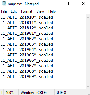
## select the maps you want to aggregate and save it into a text file using notepad.(see below screenshot)
## Assuming the file with map names is maps_aeti.txt
## below code aggregate the maps using the function "sum"
r.series file=maps_aeti.txt out=AETI_annual_2017_18 method=sum
## List all the PCP scaled maps in Grass mapset
g.list rast mapset=. pattern=L1_PCP*scaled|cat
## select the maps you want to aggregate and save it into a text file using notepad.(see below screenshot)
## Assuming the file with map names is maps_pcp.txt
## below code aggregate the maps using the function "sum"
r.series file=maps_pcp.txt out=PCP_annual_2017_18 method=sum
## press enter

Input text file with input map names

Step 4: Univariate statistics

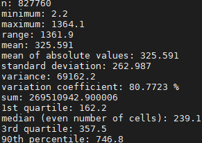
Let us now find the univariate statistics of the Annual AETI and PCP maps


# Compute univariate statistics of the annual maps
r.univar -e AETI_annual_2017_18
r.univar -e PCP_annual_2017_18
## press enter

Univariate statistics results of annual AETI 2017/18

Step 5: Find the land cover area

Let us now find the surface area of each land cover type in ULB as per WaPOR LCC map of 2018.


## Set the region to ULB
g.region vect=ulb res=250 -a
## Apply a mask to restrict further analysis to ULB
r.mask vect=ulb --o
# First list all the LCC maps
g.list rast mapset=. pattern=L1_LCC*|cat
# First let us assign category names to each land cover id as per WaPOR Catalog
# https://wapor.apps.fao.org/catalog/WAPOR_2/1/L1_LCC_A
# A text file with category details are developed and provided to you as 'rules_lcc.txt' inside 'Base_layers' folder.
r.category map=L1_LCC_2018 rules=rules.txt sep=comma
# Below command compute the surface area of each Land cover type in hectares.
r.report L1_LCC_2018 units=k -e -n -h

Step 6: Find the AETI and PCP stats per Land cover type

Let us now find the Mean and median annual AETI and PCP per land cover type.


## Set the region to ULB
g.region vect=ulb res=250 -a
## Apply a mask to restrict further analysis to ULB
r.mask vect=ulb --o
# Use the below univar command with zones and -t flag to compute stats per land cover type
# For Annual AETI
r.univar -t AETI_annual_2017_18 zones=L1_LCC_2018 sep=, output=AETI_stats_2017_18.csv
# For Annual PCP
r.univar -t PCP_annual_2017_18 zones=L1_LCC_2018 sep=, output=PCP_stats_2017_18.csv

Step 7: Assign colors and prepare map layouts

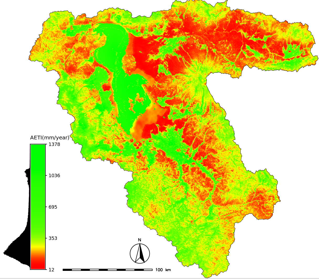
Once you have the annual AETI and PCP maps, you can assign meaningful palette to the maps and make a map layout.

To apply a color palette in GRASS GIS, a module called r.colors is used.
For setting a layout we can use the user interface commands of GRASS GIS:
Display a monitor
Display a raster in the monitor
Display a vector map
Add raster legend
Add North arrow
Add scale

In the below code snippet, let us create a nice layout for annual AETI and PCP maps


## Set the region to ULB
g.region vect=ulb res=250 -a
## Apply a mask to restrict further analysis to ULB
r.mask vect=ulb --o
## Assign a color palette to Annual AETI map
## below note that the color palette is inverted with (-n) flag and applied histo equalization using (-e) flags
r.colors -n -e map=AETI_annual_2017_18 color=gyr
## Assign a color palette to Annual AETI map
r.colors map=PCP_annual_2017_18 color=precipitation

## Create map layout for annual AETI
# Open a monitor
d.mon wx0
# erase everything in the monitor
d.erase -f
# Display a raster map
d.rast map=AETI_annual_2017_18
# Display a vector map
d.vect map=ulb type=boundary
# Add raster legend
d.legend -t -d raster=AETI_annual_2017_18 title="AETI(mm/year)" title_fontsize=20 font=sans fontsize=18
# Add North arrow
d.northarrow style=1b text_color=black
# Add Scale
d.barscale units=kilometers label=km

# Before creating the next map layout erase everything in wx0 monitor
d.erase -f

# Now Create map layout for annual PCP
# Display a raster map
d.rast map=PCP_annual_2017_18
# Display a vector map
d.vect map=ulb type=boundary
# Add raster legend
d.legend -t -d raster=PCP_annual_2017_18 title=AETI title_fontsize=20 font=sans fontsize=18
# Add North arrow
d.northarrow style=1b text_color=black
# Add Scale
d.barscale units=kilometers label=km

d.barscale will not work in Lat/Lon locations as the horizontal scale distance changes with latitude. Try d.grid instead.

Annual AETI map

Step 8: Export the maps to Geotiff format

Once you have the annual AETI and PCP maps, it might be useful to have them in other formats like Geotif (.tif). With raster maps in .tif format, you can open them in any other software like QGIS to create map layouts or further analysis


## navigate to the output folder where you want the exported raster maps in tif format
cd /mnt/path/to/outputfolder
g.region vect=ulb res=250 -a
## Apply a mask to restrict further analysis to ULB 
## If a mask is applied the exported map will be also clipped to the mask
r.mask vect=ulb --o
# Use the below commands to export the annual AETI and PCP to geotiff (.tif)
# For Annual AETI
r.out.gdal in=AETI_annual_2017_18 out=AETI_annual_2017_18.tif
# For Annual PCP
r.out.gdal in=PCP_annual_2017_18 out=PCP_annual_2017_18.tif

Your tasks

Follow the above steps (3-6) to compute Annual AETI and PCP maps for the years 2018/19 and 2019/20.

Compute univariate statistics of Annual AETI and PCP of crop years 2018/19 and 2019/20
Compute Landcover based statistics of Annual AETI and PCP of crop years 2018/19 and 2019/20
Prepare maps of Annual AETI and PCP with a nice layout (in QGIS?)
Submit a short report (max 3 pages) with the results in OCW platform midnight 12 July 2021

Last changed: 2021-07-07

Licensed under a Creative Commons Attribution-ShareAlike 4.0 International License - Thanks to Vaclav Petras for the style.