Spatio-temporal analysis with GRASS GIS

IHE Delft Institute for Water Education

The Netherlands

Outline

Exercise 2 - Spatio-temporal analysis of climatic data

In this session, we will go through the most commonly used spatial analysis techniques in GRASS GIS. The session is a hands-on with a common exercise which covers basic raster processing capabilities of GRASS GIS.

Data

Aggregated ECA&D climatic data: monthly data of 30 years averages, 0.25° resolution
Related elevation model
NaturalEarth Admin0 country borders

Data download

For this exercise, we will use some GeoTIFF files and the GRASS GIS location "ecad_ll"

Download the GeoTIFF files here
Download the GRASS GIS location here
Unzip the "grassdata_ecad_LL.zip" into "D:/grassdata" folder

Workflow overview

How do we work with spatial data in GRASS GIS?

Assuming we already have our maps in the GRASSDBASE (i.e., grassdata/location/mapset), the first step is to import the datasets to GRASS GIS. We will import the elevation data required for the exercise, and the rest of the data is already imported to the GRASS GIS mapset ecad50.

Spatial data analysis with GRASS GIS

Download the shared data. Copy the given GRASS GIS location to this path: D:/grassdata. There are two mapsets in the provided location "ecad_ll":

PERMANENT
ecad50 - Where all the ECAD datasets are stored

We will now create a new mapset "user1" in the same location "ecad_ll" to do all our analysis. To make use of the ecad dataset, we will add the mapset "ecad50" in the search path. We can run the commands from the command line or use the main GUI and copy the corresponding commands for future replication of the workflow. Note the "Copy" button in the GUI of each module. Maybe you might want to get help about the options and flags of the different commands, e.g. r.colors --help

 
        
# Launch GRASS GIS, -c creates new mapset user1, --gui launches the gui
grass78 /mnt/d/grassdata/ecad_ll/user1/ -c --text
# set the region to default
g.region -d
# List all the raster maps in all the mapsets in the search path
g.list type=rast 
# List all the mapsets in the search path
g.mapsets -p
# List all the mapsets in the location
g.mapsets -l
# Add the mapset ecad50 to the search path
g.mapsets mapset=ecad50 operation=add
# List all the mapsets in the search path
g.mapsets -p
# List all the raster maps in all the mapsets in the search path
g.list type=rast

Import data into GRASS GIS

We will now import the elevation map, provided as a GeoTIFF to the current mapset. Then set the color palette to elevation


        
# Change dirctory to the one with TIFF files
cd /d/ecad5_geotiffs_LL
# Import the elevation raster map in GeoTIFF format into GRASS GIS
r.in.gdal input=elev_0.25deg_reg_v6.0.tif output=elev_ecad
# Set the color palette of the elevation raster map to 'elevation'
r.colors map=elev_ecad color=elevation

Visualize data

Let us now display the elevation map and add decorations.

 
# Open a monitor
d.mon wx0

# Display a raster map
d.rast map=elev_ecad

# Display a vector map
d.vect map=country_boundaries type=boundary

# Add raster legend
d.legend -t -s -b raster=elev_ecad title=ELEVATION title_fontsize=20 font=sans fontsize=18

# Add North arrow
d.northarrow style=1b text_color=black

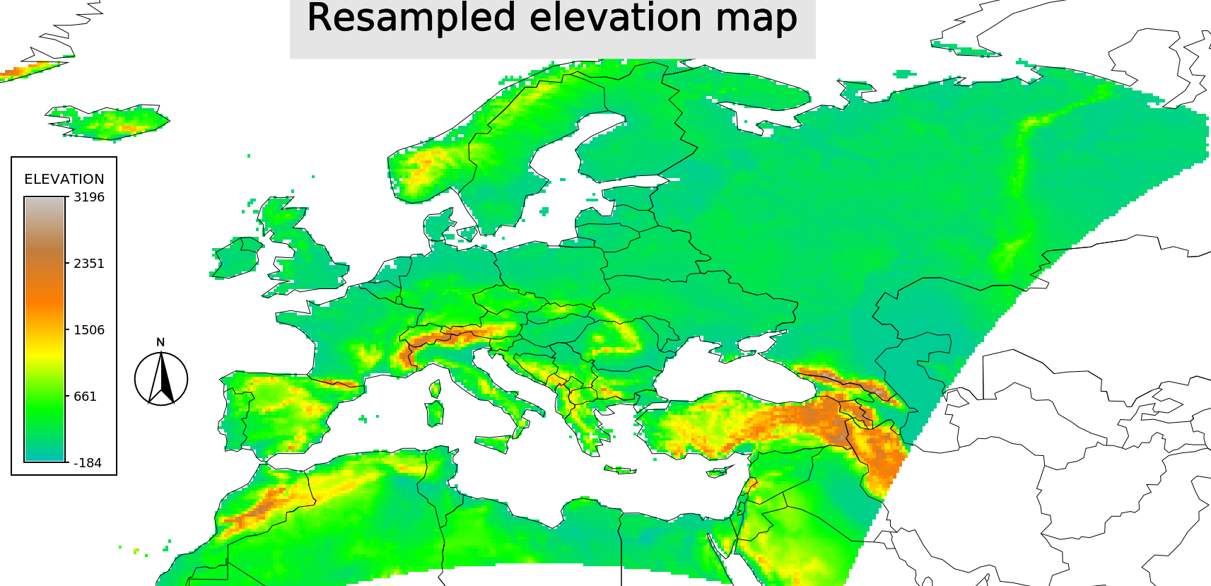
Elevation in meters

Data aggregation in GRASS GIS

Let us check how to aggregate multiple maps at different time periods based on different statistical methods

Let us create the following aggregated maps:

annual precipitation for 1951-1980 and 1981-2010
mean annual temperature for 1981-2010
minimum annual temperature for 1981-2010


        
# Set the computational region
g.region rast=precip_0_25deg_1951_1980_monthly_sums.01
# Display the region
g.region -p
# list all monthly maps for the period 1951-1980 needed for the annual precipitation aggregation
g.list rast pattern="precip_0_25deg_1951_1980_monthly_sums.*"
# Now use the r.series command to create annual precip for the period 1951 to 1980
r.series in=`g.list rast pattern="precip_0_25deg_1951_1980_monthly_sums.*" sep=","` out=precip_0_25deg.1951.1980.sum method=sum
# Set the color
r.colors precip_0_25deg.1951.1980.sum col=precipitation
# list all monthly maps for the period 1981-2010 needed for the annual precipitation aggregation
g.list rast pattern="precip_0_25deg.1981_2010.*"
# Now use the r.series command to create annual precip for the period 1981 to 2010
r.series in=`g.list rast pattern="precip_0_25deg.1981_2010.*" sep=","` out=precip_0_25deg.1981.2010.sum method=sum
# Set the color
r.colors precip_0_25deg.1981.2010.sum col=precipitation
# Aggregate the temperature maps average annual temperature
r.series in=`g.list rast pattern="tmean_0_25deg.1981_2010*" sep=","` out=tmean_0_25deg.1981_2010.avg method=average
# Set the color
r.colors tmean_0_25deg.1981_2010.avg col=celsius

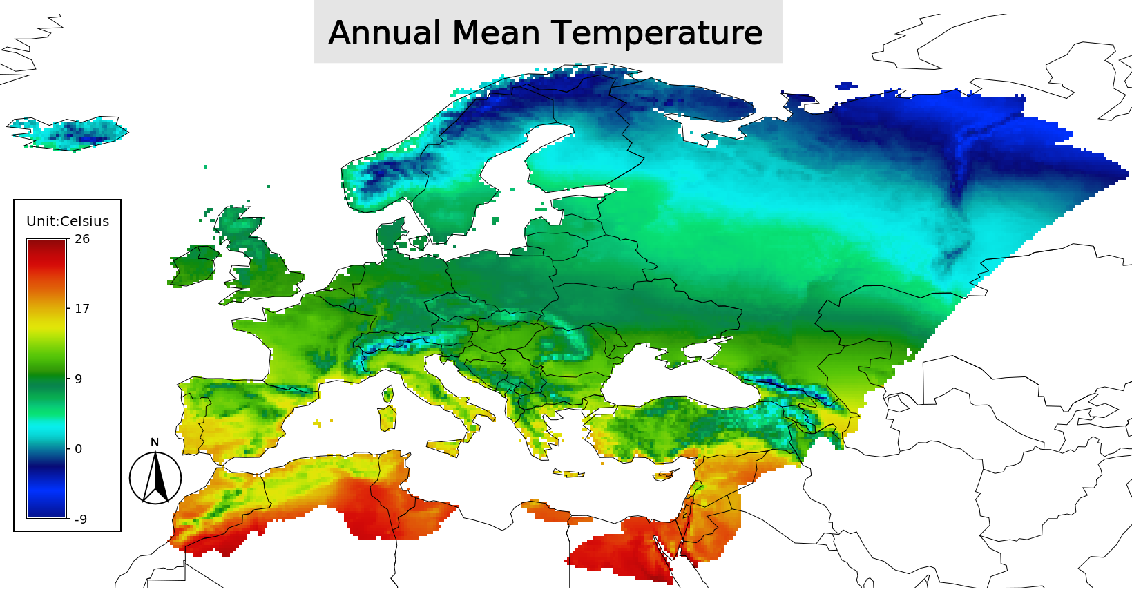
Annual Mean temperature (1981 - 2010)

Task:Now try aggregating the mean temperature maps for the period 1951 to 1980 to create annual mean temperature for the same period. Display the annual precipitation and temperature maps with legend and compare the legends using WxGUI or d.mon. For more details on r.series check here.

Univariate statistics in GRASS GIS

Now lets compute univariate statistics of the developed annual maps over the entire area and also over a particular country.


        
# Compute extended univariate statistics
r.univar tmean_0_25deg.1981_2010.avg -e -g
# Compute extended univariate statistics
r.univar precip_0_25deg.1981.2010.sum -e -g
# Get a feel of the vector data and the attributes
v.db.select country_boundaries|head -5
# Find the attributes related to The Netherlands
v.db.select country_boundaries|grep Netherlands
# Mask out all the area other than The Netherlands
r.mask vect=country_boundaries cats=118
# Repeat the univariate statistics for The Netherlands
r.univar tmean_0_25deg.1981_2010.avg -e -g
# Repeat the univariate statistics for The Netherlands
r.univar precip_0_25deg.1981.2010.sum -e -g
# Remove the mask
r.mask -r

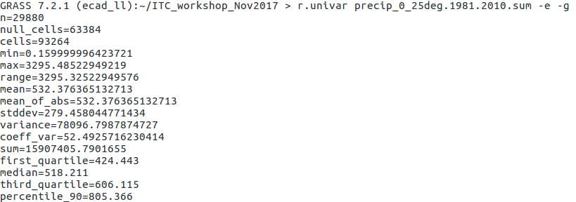
Univariate statistics of annual precipitation (1981 to 2010)

Raster map algebra using map calculator

Let us compute a difference map from the two 30 years aggregated precipitation maps.


        
# we want to be sure to have the computational region set			
g.region rast=precip_0_25deg.1981_2010.06.sum -p
# Map algebra using map calculator
r.mapcalc "diff_1951_1981_2010 = precip_0_25deg.1951.1980.sum - precip_0_25deg.1981.2010.sum"
# apply inverse “differences” color table
r.colors raster=diff_1951_1981_2010 color=differences
# Now lets convert all the tmean maps into kelvin
# For that we need to apply the same equation to 24 maps.
g.list rast pattern=tmean*
g.list rast pattern=tmean* |wc -l
# Lets do it using a for loop
for i in `g.list rast pattern=tmean*`; do 
	r.mapcalc "${i}.Kelvin = ${i} + 273.15"
done
# Now check if the maps are there
g.list rast pattern=tmean*Kelvin
# set the colors 
for i in `g.list rast pattern=tmean*Kelvin`; do 
	r.colors map=${i} color=kelvin
done

Task:Visualize the difference map with the legend and compute univariate statistics over The Netherlands.

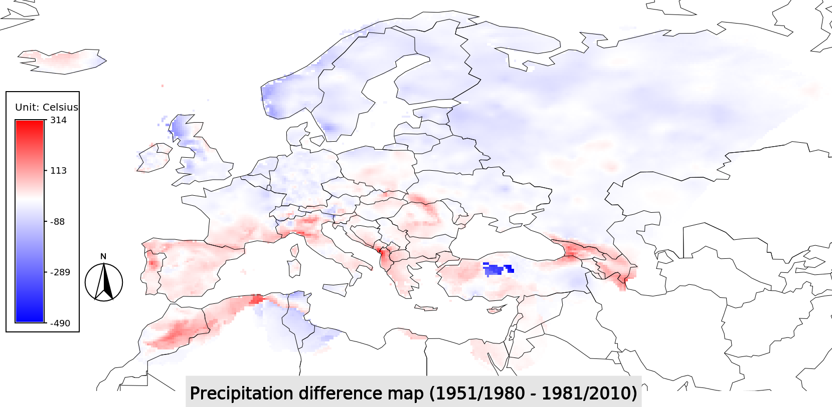
Difference between precipitation (1951-1980) and (1981-2010)

Zonal statistics in GRASS GIS

We want to extract a table with basic statistics over all the countries in Europe.

Main steps are:

Explore the attributes of the vector data
Rasterize the vector data
Generate zonal statistics based on r.univar


        
# check the available column (or use wxGUI attribute manager)
v.info -c country_boundaries
# look at country names
v.db.select country_boundaries column="NAME"
# we want to be sure to have the computational region set	
g.region rast=precip_0_25deg.1981.2010.sum -p
# for zonal statistics, we convert the vector polyons to raster model
v.to.rast country_boundaries out=country_boundaries use=cat labelcolumn="NAME"
# check raster polygons
r.category country_boundaries
# get the statistics for each country as a table
r.univar -t precip_0_25deg.1981.2010.sum zones=country_boundaries sep="," output=countries_precip_1981_2010_sum.csv
r.univar -t diff_1951_1981_2010 zones=country_boundaries sep="," output=countries_precip_1951_1980_vs_1981_2010_sum.csv

Extract data

Let us see how to extract raster values at particular observation points given as a vector layer. Here we will first create a simulated observation points using random sampling.

 
# Create 10 random points over the computational region
r.random input=tmean_0_25deg.1981_2010.avg n=10 vector=obs_points
# Extract raster tmean 1981-2010 avg values at these 10 points
r.what -n map=tmean_0_25deg.1981_2010.avg points=obs_points sep=comma output=extract_single.txt
# Now extract values from multiple raster maps
r.what -n map=`g.list rast pattern="tmean_0_25deg.1981_2010*" sep=comma` points=obs_points sep=comma output=extract_multiple.txt

Task:Check now the module v.what.rast and find out how to query and add raster value into the vector map attribute table.

Time series analysis

In this session, let us see how to create a temporal data base to store time series data. We will create an empty database and then add monthly maps to it.

 
# For windows user, add scripts path in the Power Shell
export PATH=/c/OSGeo4W64/apps/grass/grass-7.4.0/scripts:$HOME/AppData/Roaming/GRASS7/addons/scripts:$PATH
# Ignore the sqlite warnings in the following commands
# Create an empty temporal database (STRDS) for storing the monthly long term average maps from 1951 to 1980
t.create.py output=tmean_monthly_1951_1980.avg type=strds semantictype=mean temporaltype=absolute title="monthly tmean 1951 to 1980 avg" description="monthly tmean 1951 to 1980 avg"
# Create a text file with map names in order which has to be registered in the created database (STRDS)
g.list -m rast pattern=tmean*1951_1980*Kelvin >> filenames_tmean1.txt
# Register the maps to the created temporal database (STRDS)
t.register.py -i input=tmean_monthly_1951_1980.avg type=rast file=filenames_tmean1.txt start=1980-01-01 increment="1 months" --o
# List the maps in the temporal database (STRDS)
t.rast.list.py tmean_monthly_1951_1980.avg
# Univariate statistics of all the maps in the STRDS and save to a text file
t.rast.univar.py tmean_monthly_1951_1980.avg sep=comma >> univar_stats_tmean_1951_1980.txt
# Aggregate to 1 year
t.rast.aggregate.py input=tmean_monthly_1951_1980.avg output=tmean_annual_1951_1980.avg basename=tmean_annual_1951_1980.avg granularity="1 years" method=average where="start_time >= '1980-01-01'"
# Aggregate to 3 months
t.rast.aggregate.py input=tmean_monthly_1951_1980.avg output=tmean_seasonal_1951_1980.avg basename=tmean_seasonal_1951_1980.avg granularity="3 months" method=average where="start_time >= '1980-01-01'"

Task: Repeat the above step and create a new STRDS for monthly tmean maps from 1981 to 2010.

Map algebra using temporal STRDS

Temporal algebra is powerful way of executing different equations with multiple temporal databases. For example if we want to compute the difference between long term monthly averages in the period 1951-1980 and 1981-2010, It can be done in one step using TGRASS module. You need to finish the above task to do the following step.

 
# For windows user, add scripts path in the Power Shell
export PATH=/c/OSGeo4W64/apps/grass/grass-7.2.2/scripts:$PATH
# Ignore the sqlite warnings in the following commands
# Create a new temporal database (STRDS) of difference maps between monthly maps of period 1951-1980 and 1981-2010
# Make sure you already have created the STRDS "tmean_monthly_1981_2010.avg"
t.rast.mapcalc.py input=tmean_monthly_1951_1980.avg,tmean_monthly_1981_2010.avg expression="tmean_monthly_1951_1980.avg - tmean_monthly_1981_2010.avg" output=tmean_monthly_diff.avg basename=tmean_monthly_diff.avg
# Check the list raster maps in the new STRDS
t.rast.list.py tmean_monthly_diff.avg
# Univariate statistics of all the maps in the STRDS and save to a text file
t.rast.univar.py tmean_monthly_diff.avg sep=comma >> univar_stats_tmean_diff_avg.txt

Task: Extract the raster map values from the temporal database "tmean_monthly_diff.avg" from the observation points created in the above section using t.rast.what

Cluster analysis in GRASS GIS

Let us now do climatic characterisation of Europe using unsupervised classification

Main steps are:

Group the images
Generate signatures using a clustering algorithm
Classify using maximum likelihood algorithm


        
# pick the variables of interest
g.list rast pattern="*_0_25deg.1981_2010.*.*"
# add maps to an imagery group for easier management
i.group group=ecad_1981_2010 subgroup=ecad_1981_2010 input=`g.list rast pattern="*_0_25deg.1981_2010.*.*" sep=","`
# statistics for unsupervised classification
i.cluster group=ecad_1981_2010 subgroup=ecad_1981_2010 sig=ecad_1981_2010 classes=5 separation=0.5
# Maximum Likelihood unsupervised classification
i.maxlik group=ecad_1981_2010 subgroup=ecad_1981_2010 sig=ecad_1981_2010 output=ecad_1981_2010.class rej=ecad_1981_2010.class.rej

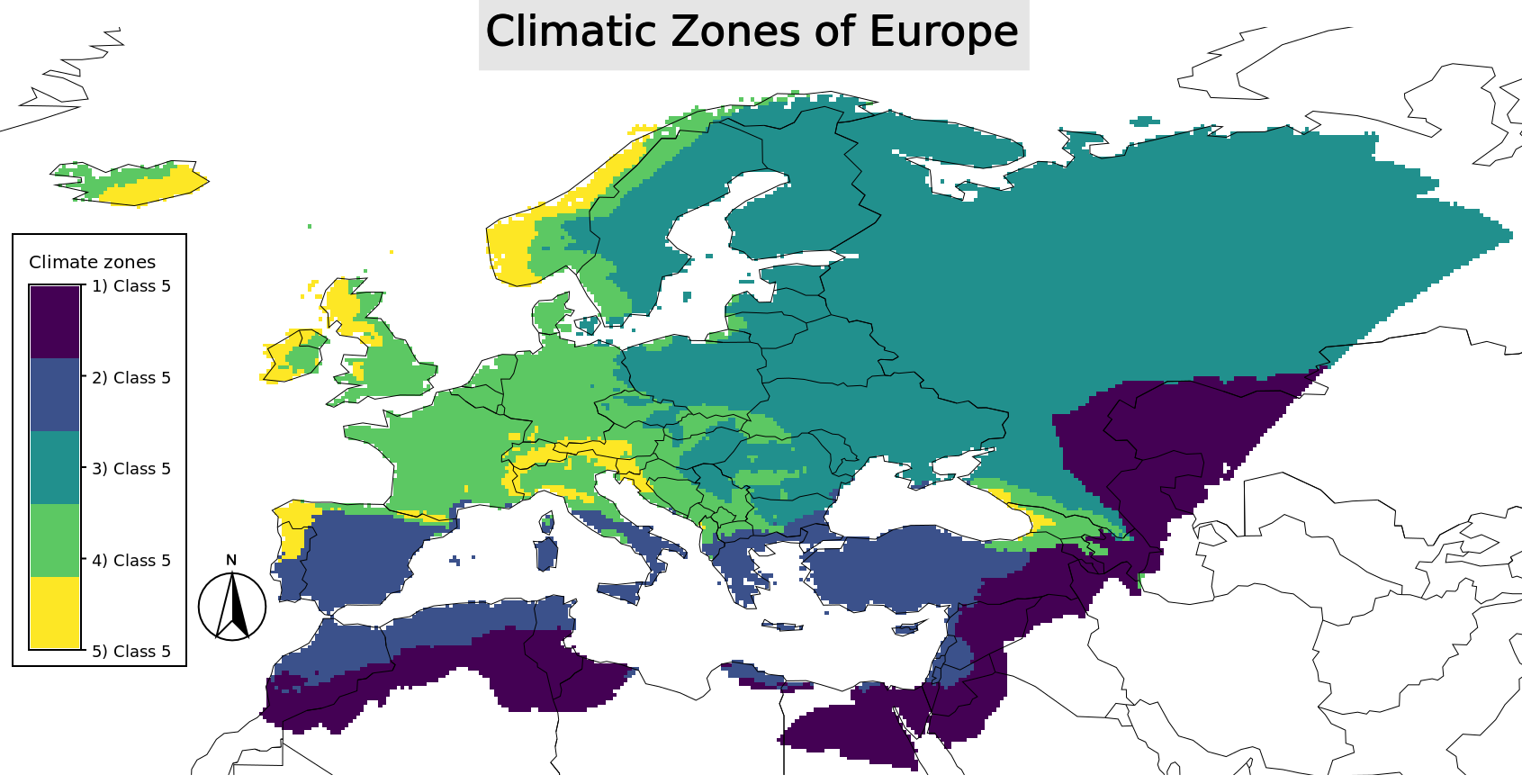
Climatic Zones of Europe

Check the manual of i.cluster and i.maxlik.

Check if the result make sense comparing to the Kottek, M. et al., 2006

Linear models in GRASS GIS

Let us now look at the relation ship between mean temperature, elevation and latitude.


        
# Create a latitude map
r.mapcalc "latitude = y()"
# linear regression model
r.regression.line mapx=elev_ecad mapy=tmean_0_25deg.1981_2010.avg
# Apply the model using the model variables
r.mapcalc "tmean_model_line = 6.143929 + 0.002434 * elev_ecad"
# Calculate a difference map
r.mapcalc "tmean_model_diff_line = tmean_model_line - tmean_0_25deg.1981_2010.avg"
# Apply differences color palette
r.colors tmean_model_diff_line color=differences
# Multiple linear regression model
r.regression.multi mapx=elev_ecad,latitude mapy=tmean_0_25deg.1981_2010.avg
# Apply the model using the model variables
r.mapcalc "tmean_model_multi = 40.722804 + -0.004234 * elev_ecad + -0.629130 * latitude"
# Calculate a difference map
r.mapcalc "tmean_model_diff_multi = tmean_model_multi - tmean_0_25deg.1981_2010.avg"
# Apply differences color palette
r.colors tmean_model_diff_multi color=differences

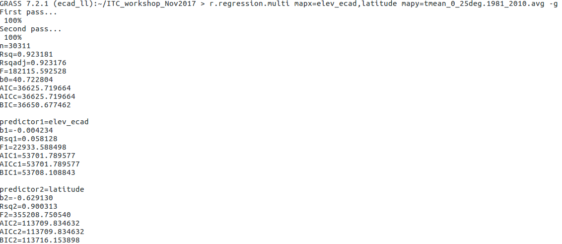
Multiple linear regression model

Visualize the model outputs and difference maps. Please check the manual of r.regression.line and r.regression.multi.

To use R functionalities inside GRASS GIS making use of the datasets in the mapset refer here

Interpolation in GRASS GIS

GRASS GIS offers a wide range of interpolation algorithms. List of interpolation methods available in GRASS GIS are given here


        
# set the region
g.region rast=elev_ecad -p
# extract 500 random points
r.random input=tmean_0_25deg.1981_2010.avg n=500 vector_output=t_mean_europe_meteo 
# open a monitor
d.mon wx0
# visualize the raster and vector maps with a grid
d.rast tmean_0_25deg.1981_2010.avg
d.vect t_mean_europe_meteo icon=basic/circle
d.grid 10
# set the sea mask to avoid interpolation over sea
r.mapcalc "sea = if(isnull(elev_ecad), 1, null() )"
r.mask -i sea
# check the attributes of the random points
v.info -c t_mean_europe_meteo
# Apply IDW interpolation
v.surf.idw t_mean_europe_meteo output=t_mean_europe_meteo_idw column=value
# Apply celsius color palette
r.colors t_mean_europe_meteo_idw color=celsius
# Apply Spline interpolation
v.surf.rst t_mean_europe_meteo elev=t_mean_europe_meteo_rst layer=1 zcolumn=value
# Apply celsius color palette
r.colors t_mean_europe_meteo_rst color=celsius
# remove mask
r.mask -r

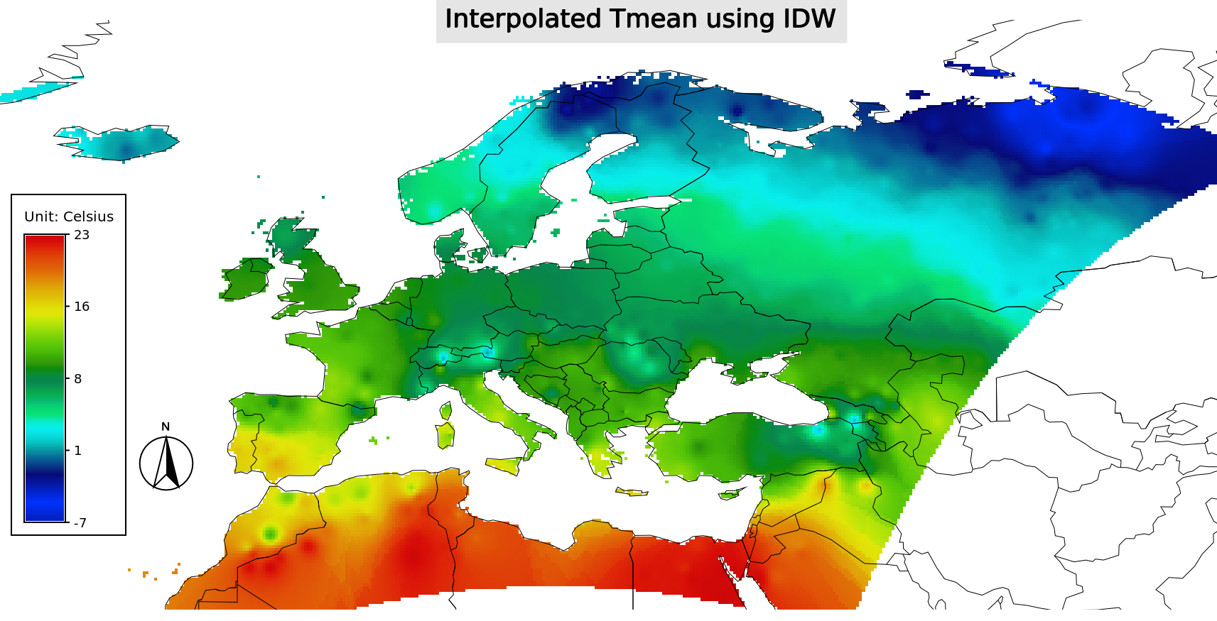
IDW interpolated map of Tmean

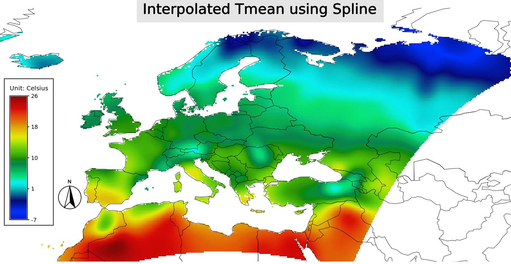
Spline interpolated map of Tmean

Raster data export from GRASS GIS

Raster module r.out.gdal are used to export raster data from GRASS GIS to different formats. The formats supported are listed here and depends upon the GDAL installation.

        
#Export the raster map tmean_0_25deg.1981_2010.avg  into geotiff format
r.out.gdal input=tmean_0_25deg.1981_2010.avg  output=tmean_0_25deg.1981_2010_avg.tif

This tutorial is adapted from Geostat exercises prepared by Markus Neteler and related content can be found in his blog .

Last changed: 2021-07-07

Licensed under a Creative Commons Attribution-ShareAlike 4.0 International License - Thanks to Vaclav Petras for the style.