Spatio-temporal analysis with GRASS GIS

IHE Delft Institute for Water Education

The Netherlands

Outline

Introduction to GRASS GIS

Working with GRASS GIS is not much different than any other GIS. Just a few commonly used terms need to be introduced first.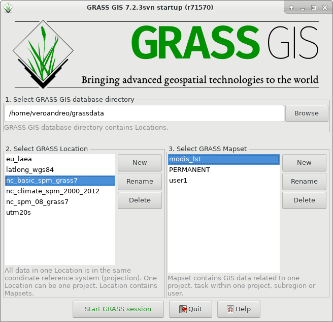

GRASS GIS start screen: GRASS database, Location and Mapset

Basic concepts: GRASS DATABASE, LOCATION and MAPSET

The GRASS DATABASE (also called "GISDBASE") is an existing directory which contains all GRASS GIS projects. These projects are organized in subdirectories called LOCATIONs.
A LOCATION is defined by its coordinate system, map projection and geographical boundaries. All data within one Location has the same coordinate reference system.
MAPSETs are subdirectories within Locations. In a MAPSET you can organize GIS maps thematically, geographically, by project or however you prefer. Mapsets can also be named after users, for example.

Within each Location, a mandatory PERMANENT mapset exists. This mapset can contain commonly used data such as base maps. The PERMANENT mapset also contains metadata related to the Location it belongs to, e.g. its projection. When GRASS GIS is started, it connects to a Database, Location and Mapset specified by the user.

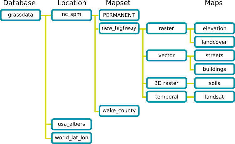
GRASS DATABASE, LOCATIONs and MAPSETs

Why this structure?

GRASS GIS has a native format for raster and vector data, therefore they must be imported (r|v.import, r.in.gdal, v.in.ogr, among others) or linked (r|v.external) into a GRASS Location/Mapset.

What are the advantages?

GRASS DATABASE, LOCATIONs and MAPSETs are folders that can be easily (zipped and) shared with other users. The latter just need to (unzip and) move into their GRASS DATABASE (and proper location in case of sharing a mapset).
The GRASS DATABASE can be local or remote, and special permissions can be set to specific mapsets in a LOCATION (the PERMANENT mapset is accessible from all other mapsets and users).
Since all data in a LOCATION have necesarily the same CRS, the problem of non-matching map projections, often encountered in other GIS programs, does not exist.

Further details can be found at the GRASS database manual page.

Data formats supported

GRASS GIS is able to read most raster and vector data formats directly (mainly done through the GDAL/OGR library). As mentioned above, GRASS GIS has its own internal formats to manage raster and vector data, therefore your data have to be imported or linked into a GRASS LOCATION/MAPSET for further processing and analysis.

Unlike other GIS, GRASS GIS native vector format is topological, this means that adjacent geographic components in a single vector map are related to each other. For example, in a non-topological GIS if two areas share a common border that border would be digitized twice and also stored in a duplicate manner. In a topological GIS such as GRASS GIS, this border exists only once and it is shared between these two areas. The topological representation of vector data helps to produce and maintain vector maps with clean geometry. Moreover, it enables certain analyses that can not be conducted with non-topological or spaghetti data.

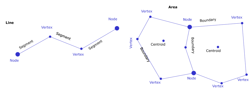
Vector data types in GRASS GIS

Data types in GRASS GIS

GRASS GIS can handle the data types listed below. Follow the links for more detailed descriptions of these data types, how they are implemented in GRASS GIS, and how to work with them.

Raster (including satellite imagery)
3D raster or voxel
Vector: point, line, boundary, area, face
Space-time datasets: collections of raster (STRDS), raster 3D (STR3DS) or vector (STVDS) maps

Modules

GRASS functionality is available through modules (aka tools or functions). GRASS GIS is composed of more than 500 modules to perform any kind of GIS analysis. It is possible to analize raster, raster 3D, imagery and vector maps along with their alphanumerical attributes. Modules respect the following naming conventions:

GRASS GIS module families
Prefix	Function class	Type of command	Example
g.*	general	general data management	g.rename: renames map
d.*	display	graphical output	d.rast: display raster map, d.vect: display vector map
r.*	raster	raster processing	r.mapcalc: map algebra, r.univar: univariate statistics
v.*	vector	vector processing	v.clean: topological cleaning
i.*	imagery	imagery processing	i.pca: Principal Components Analysis on imagery group
r3.*	voxel	3D raster processing	r3.stats: voxel statistics
db.*	database	database management	db.select: select value(s) from table
ps.*	postscript	map creation in PostScript format	ps.map: PostScript map creation
t.*	temporal	space-time datasets	t.rast.aggregate: raster time series aggregation

These are the main groups of modules. Some modules have multiple dots in their names. This often suggests further grouping. For example, modules staring with t.rast.* deal with time series of raster data.

The name of the module always relates to its function. For example, v.in.lidar starts with v so it deals with vector maps; the second part of the name is in which indicates that the module is for importing data into GRASS GIS and finally, the name ends in lidar indicating that it deals with lidar point clouds.

The graphical user interface (GUI) offers a module tree view as well as a module search engine to find the function you need either by browsing through the tree or typing the name or part of the name of a module in the search box.

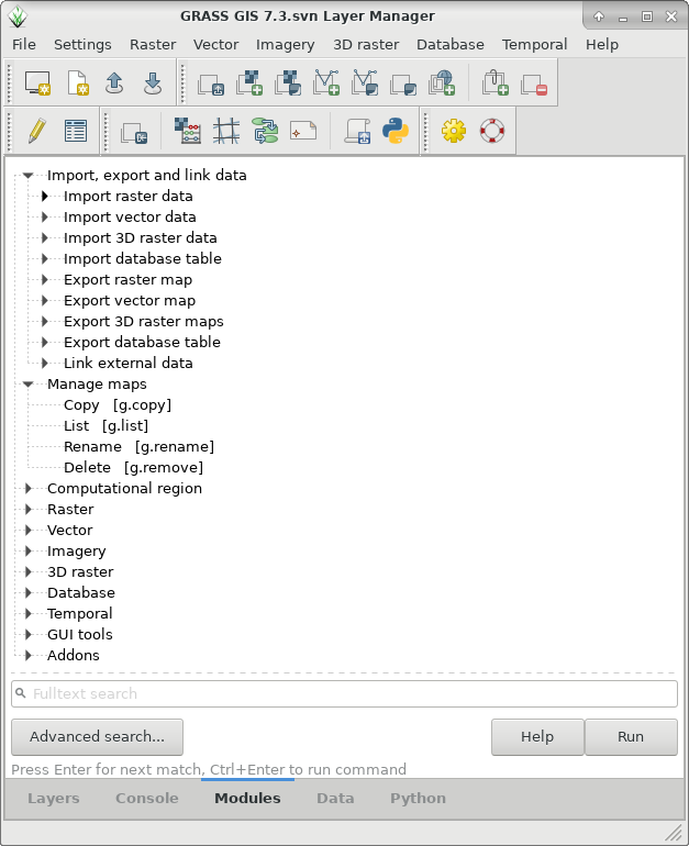
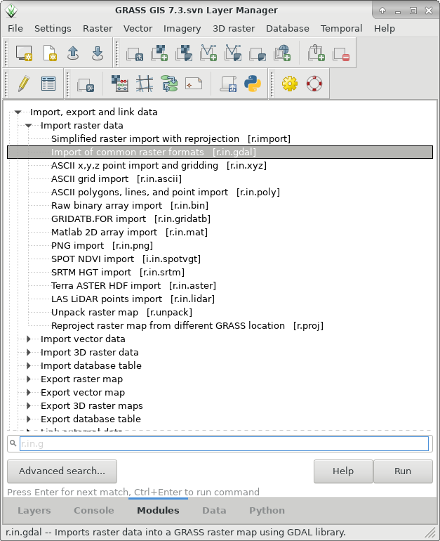
Module tree and search engine

It is also possible to install further modules, called Add-ons, from a centralized GRASS GIS Add-on repository at OSGeo or from github (or similar repositories) using the command g.extension. In the official GRASS GIS Add-on repository there are more than 300 modules that notably extend the capabilities of GRASS GIS.

		
# install extension from GRASS GIS Add-on repository
g.extension extension=r.hants

# install extension from github repository
g.extension url=https://github.com/pesekon2/GRASS-GIS-SOS-tools/tree/master/sos/r.in.sos

Computational region

The computational region is a cornerstone concept in GRASS GIS: it is the actual setting of the region boundaries and the actual raster resolution. If you want to be able to use GRASS to its full potential, you have to understand it. In fact, it is so important that you should know about it even if you only plan some light usage of GRASS.

The raster input maps are automatically (on the fly) cropped/padded and rescaled to match the current region, the output maps have their bounds and resolution equal to those of the current computational region, while vector maps are always considered completely.

Before we use a module to compute a new raster map, we must set the computational region properly. All raster computations will be performed in the current region settings, i.e. the current region extent and current raster resolution. If the resolution differs from that of the input raster map(s), on-the-fly resampling is performed (nearest neighbor resampling). If this is not desired, the input map(s) has/have to be resampled beforehand with one of the dedicated modules.

The computational region can be set and changed by means of g.region to the extent of a vector map (e.g. boundary of a state or county), a raster map or manually to some area of interest. Moreover you can save region settings and reload them when necessary. Besides, the region settings persist between GRASS sessions and are mapset specific.

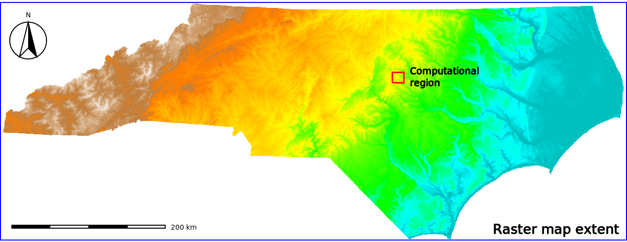
Raster map extent vs. Computational region

Which are the advantages?

keep your results consistent
avoid clipping maps
test an algorithm or computationally demanding process in small areas first
fine-tune the settings of a certain module
run different processes in different areas

A word of caution for new users: Make always sure that the region is set correctly before doing any work on your map. A typical problem of newcomers to GRASS is that they import a map, do some computations, and end up with an empty output layer. This is almost always due to wrong region settings in which the imported map falls outside the area currently covered by the region. For a more detailed explanation of the region and how to work with it, see the Wiki page about the Computational region .

Mask

Like the region, the Mask is an important concept in GRASS that you need to understand to use GRASS to its full potential. If a mask is set, raster modules will operate only on data falling inside the masked area(s), i.e. any data falling outside of the mask are treated as if their pixel values were NULL. To set the mask you can use r.mask or create a raster called MASK (this raster map name is reserved for this purpose).

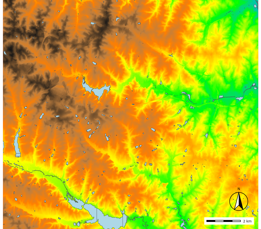
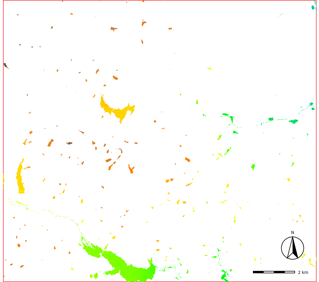
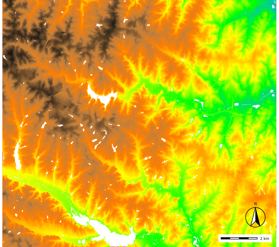
By setting the MASK (here based on lakes vector map) only the raster data inside the masked area (lakes) are used for further analysis (center). If we want to mask the lakes and analyze the rest, we create an "inverse" mask (right).

For new users, make always sure you know if/what MASK is set. You can easily check if there is a mask set by checking if there is a layer with the name MASK in your mapset. You can also display the MASK like any other raster layer. For more details about using masks, see the r.mask manual page.

Interfaces

GRASS GIS offers different interfaces for the interaction between user and software. Let's see them...

Graphical User Interface (GUI)

The GUI is the simplest way to approach GRASS GIS. It offers a user-friendly approach to executing modules where the users can navigate to data layers that they would like to analyze and modify processing options with simple check boxes. The GUI also offers an easily accessible manual on how to execute a module.

The GRASS GIS GUI is composed of two elements, the Layer Manager where you can find all the GRASS GIS modules and manage your data and, the Map Display where you can navigate, print and query your maps. The GUI also comes with a Python shell for rapid prototyping.

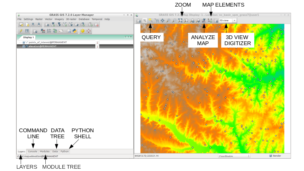
GRASS GIS Graphical User Interface (GUI)

Command line

The command line is the traditional and, probably, the most powerful way to use GRASS GIS, used daily by many GRASS GIS power users worldwide.

The command line interface allows users to execute a module using command prompts specific to that module. This is handy when you are running similar analyses with minor modification or are familiar with the module commands for quick efficient processing.

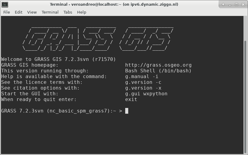
GRASS GIS command line interface

Advantages of the command line

Run "history" to see all your previous commands
History is stored individually per MAPSET
Search in history with CTRL-R
Save the commands to a file: history > my_protocol.sh, polish/annotate the protocol and re-run with: sh my_protocol.sh
Call module's GUI, set all options and "Copy" the final command for further replication

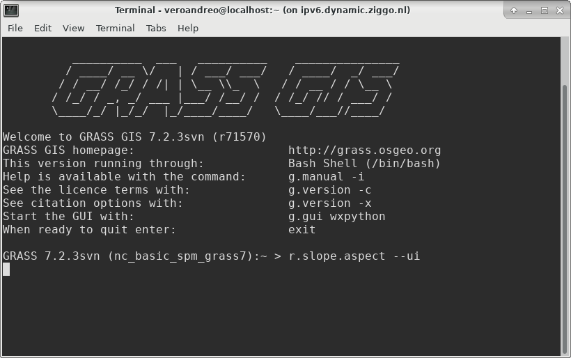
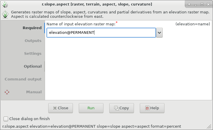
Calling a module GUI from the terminal

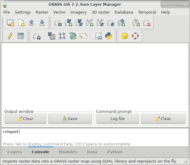
Remember that there is a simplified command line included in the GUI, the tab "Console". It offers a "Command prompt" button to save the command's history to a file.

Command line in the main GUI

Python

Python is a powerful and simple programming language, and you can use it to:

interface with the functionalities offered by GRASS GIS
create your own workflows chaining several GRASS GIS modules
create new add-ons by using GRASS GIS modules along with a wide number of Python libraries.

The simplest way to execute a Python script using GRASS GIS modules is to use the "Simple Python editor" accessible from the toolbar or the Python tab in the Layer Manager.

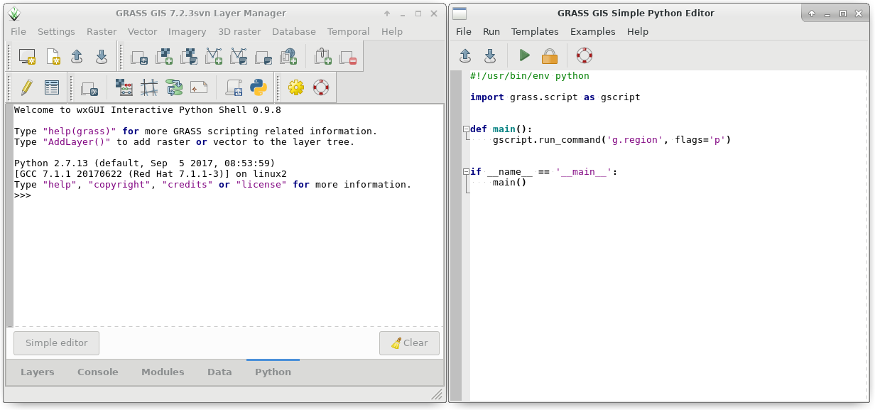
Python console and simple Python editor

Another option is to write the Python code in your favorite plain text editor. Then, run the script in GRASS GIS using the main menu File -> Launch script. Here's an example of Python code to run GRASS GIS modules:

		
!/usr/bin/env python

# simple example for pyGRASS usage: raster processing via modules approach

from grass.pygrass.modules.shortcuts import general as g
from grass.pygrass.modules.shortcuts import raster as r

g.message("Filter elevation map by a threshold...")

# set computational region
input = 'elevation'
g.region(rast=input)

# hardcoded:
# r.mapcalc('elev_100m = if(elevation > 100, elevation, null())', overwrite = True)

# with variables
output = 'elev_100m'
thresh = 100.0
r.mapcalc("%s = if(%s > %d, %s, null())" % (output, input, thresh, input), overwrite = True)
r.colors(map=output, color="elevation")

QGIS

There are two ways to use GRASS GIS and its functionalities in QGIS: through the GRASS GIS plugin and through Processing toolbox. In the first case, QGIS works as a GUI for GRASS GIS, and users can process and analyze their data in the GRASS Database with GRASS GIS modules. In the second case some of the GRASS GIS modules are available through Processing toolbox, and it allows to use GRASS functionality with data not necessarily in the GRASS Database.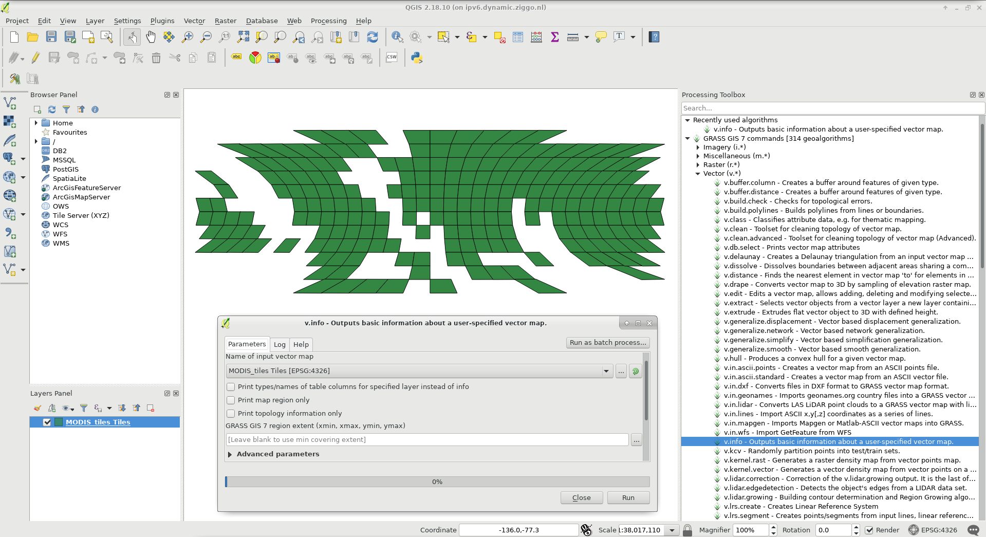

GRASS modules through Processing Toolbox

R + rgrass7

GRASS GIS and R can be used together in two ways:

Using R within a GRASS GIS session, i.e. you start R (or RStudio) from the GRASS GIS command line.
Using GRASS GIS within an R session, i.e. you connect to GRASS GIS Database from within R (or RStudio).

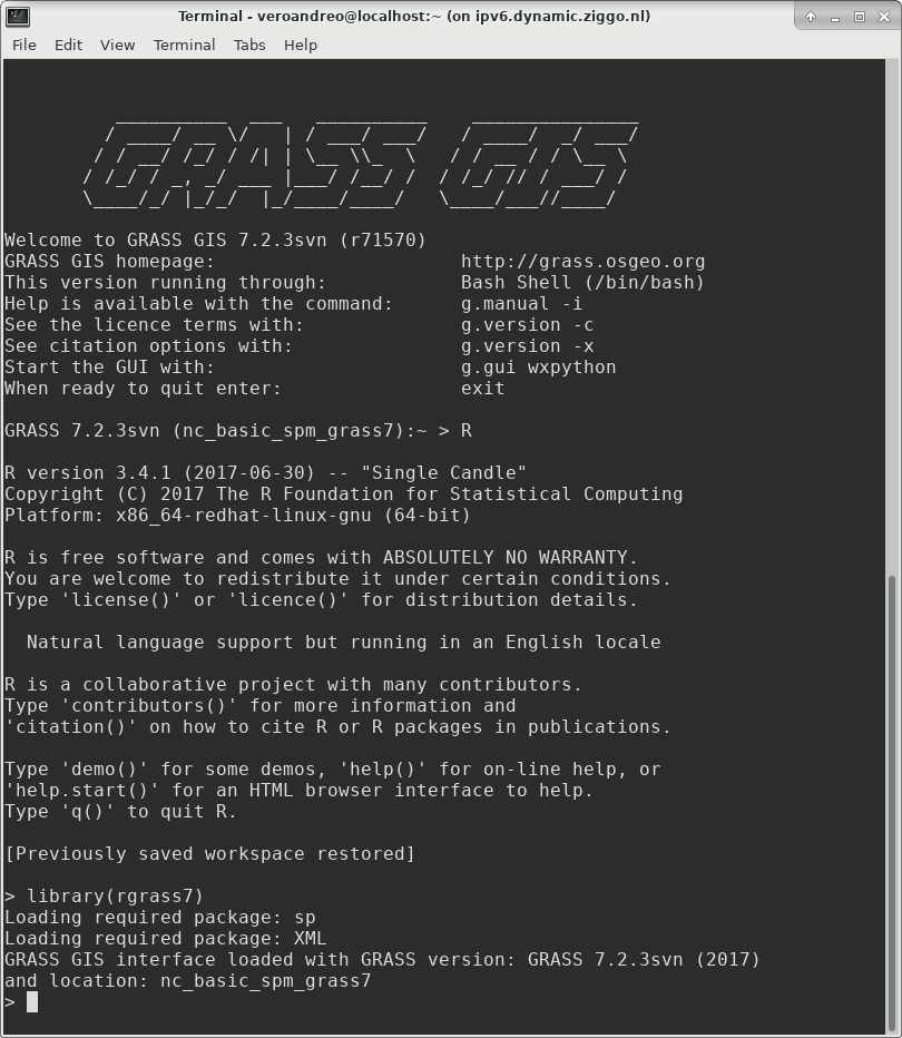
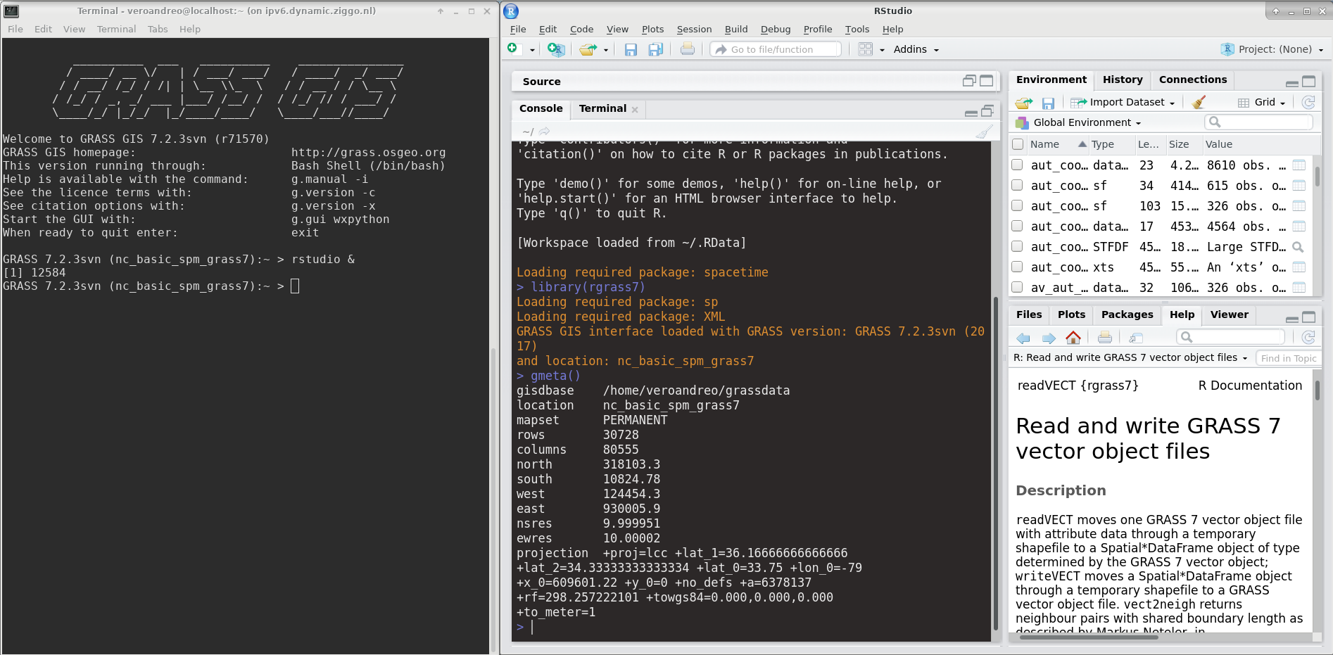
A special R package, rgrass7, provides the necessary interface to read and write data from and into GRASS Database, as well as to execute GRASS GIS commands from within R. More details and examples on both ways of combining GRASS and R can be found in the GRASS and R dedicated wiki page.

Calling R (left) and Rstudio (right) from within GRASS

WPS - OGC Web Processing Service

It is possible to run GRASS GIS modules through the web using the Web Processing Service (WPS is an OGC standard). The Free and Open Source software ZOO-Project and PyWPS allow the user to run GRASS GIS commands in a simple way.

Last changed: 2021-07-07

Licensed under a Creative Commons Attribution-ShareAlike 4.0 International License - Thanks to Vaclav Petras for the style.